Contents
Measures of Dispersion:
Dispersion denotes by how much (or to what extent) the data of a particular group are scattered from the central value.
Methods of Dispersion:
There are two different methods to study dispersion. They are:
- Mathematical Methods:
Under Mathematical Methods, we use methods like:
ii) Quartile Deviation
iii) Mean Deviation
iv) Standard Deviation
- Graphic Methods:
Mathematical Methods of Dispersion:
Quartile Deviation:
Quartile in Continuous Data Series:
Unlike Quartiles in Discrete Series, it is a little long process to find the Quartiles in continuous data series.
Continuous data series do not specify exact values. They have range of values. Example: 10-20, 20-30, 30-40, etc.
First of all, remember these notations and what they represent:
l = lower limit of the class in which the Quartile lies
N = total number of data
f = frequency of the class in which the Quartile lies
c.f. = Cumulative frequency of the class that lies just before the Quartile
i = size of the class in which Quartile lies
Sure, these above notations make no sense until we tell you these formulae:
Q1 class = (N+4)th item
Q1 = l + i/f (N/4 -c.f.)
Do you remember? Continuous data range do not specify exact values. So, first you will need to find out in which class the Q1 of that data lies in.
To find the class, use the formula: Q1 class = (N+4)th item
Now, we have the class where Q1 lies but we do not know what the Q1 is. Now, use the formula: Q1 = l + i/f (N/4 -c.f.). Replace the values of these notations with the values that you obtain from the cumulative frequency table. Then, you will find your Q1.
See the solved example to get more clear.
The same formula is with Q3, as well. Only difference is in Q3, we have 3N.
Q3 class = (3N/4)th item
Q3 = l + i/f (3N/4 -c.f.)
Interquartile Range:
Hence, interquartile range is the description of values in the middle 50% of the data set. This is written as Q3-Q1.
So, Interquartile Range = Q3 - Q1
Quartile Deviation:
Quartile Deviation is interquartile range divided by 2. This represents the dispersion of values depending upon the lower and upper quartile in the dataset.
Quartile Deviation (Q.D.) is also known as Semi-interquartile range.
Q.D. = (Q3 -Q1)/2
Coefficient of Quartile Deviation:
Formula to find coefficient of Q.D.
= (Q3 -Q1)/(Q3 +Q1)
Mean Deviation:
Mean Deviation is also known as average deviation. Mean Deviation can be calculated either from mean, median or mode. But, it gives the best result when taken from mean than others.
Remember these representations:
x̅ = Mean
M = Median
x = data
Mean Deviation about the mean:
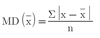
Here, x̅ represents mean, x represents the data and n represents total frequency.
Mean Deviation about the median:
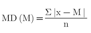
Here, M represents Median, n represents total frequency of data
Coefficient of Mean Deviation:
Coefficient of M.D. about mean:
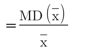
Here, MD(x̅ ) represents Mean Deviation from Mean. And, x̅ represents Mean.
Coefficient of M.D. about median:
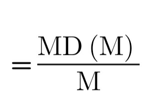
Here, MD(M) represents Mean Deviation from Median. And, M represents Median.
See the solved examples here.
Standard Deviation:
S.D. is also known as root-mean square deviation. Standard deviation is represented as 'σ' (sigma). This method of calculating dispersion measures the absolute dispersion.
Calculation of Standard Deviation:
a) Actual Mean Method:
Here, d = x-x̅ , and x̅ = actual mean, f = frequency and N = total number of observations
b) Assumed Mean Method:
Here, d = x -A, A = assumed mean, f = frequency and N = total number of observations
Here, d - m (mid-class)-A, d' = d/i , i = class interval.
Coefficient of Variation:
Hopefully these formulae will help you and to have an in-depth look over the solved examples with detailed explanations in every processes, click here.
#Statistics


0 Comments